Non Linear Relationship Scatter Plot

Measure of linear correlation

In statistics, the Pearson correlation coefficient (PCC, pronounced ) ― as well known equally Pearson'southward r , the Pearson product-moment correlation coefficient (PPMCC), the bivariate correlation,^[1] or colloquially only as the correlation coefficient ^[2] ― is a mensurate of linear correlation between two sets of data. It is the ratio betwixt the covariance of two variables and the product of their standard deviations; thus, it is essentially a normalized measurement of the covariance, such that the issue always has a value between −1 and 1. As with covariance itself, the measure can merely reflect a linear correlation of variables, and ignores many other types of relationships or correlations. As a simple example, ane would expect the historic period and elevation of a sample of teenagers from a high school to accept a Pearson correlation coefficient significantly greater than 0, merely less than 1 (as 1 would represent an unrealistically perfect correlation).

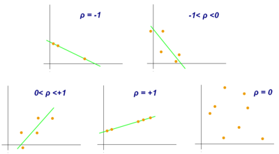
Examples of besprinkle diagrams with different values of correlation coefficient (ρ)

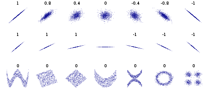
Several sets of (x,y) points, with the correlation coefficient of x and y for each ready. Note that the correlation reflects the force and direction of a linear relationship (superlative row), but non the slope of that relationship (heart), nor many aspects of nonlinear relationships (bottom). North.B.: the figure in the center has a gradient of 0 only in that case the correlation coefficient is undefined considering the variance of Y is zero.

Naming and history [edit]

Information technology was developed past Karl Pearson from a related idea introduced by Francis Galton in the 1880s, and for which the mathematical formula was derived and published past Auguste Bravais in 1844.^{[a] [six] [7] [8] [9]} The naming of the coefficient is thus an example of Stigler's Police.

Definition [edit]

Pearson's correlation coefficient is the covariance of the two variables divided by the product of their standard deviations. The form of the definition involves a "production moment", that is, the mean (the first moment near the origin) of the product of the mean-adapted random variables; hence the modifier product-moment in the name.

For a population [edit]

Pearson's correlation coefficient, when applied to a population, is commonly represented past the Greek alphabetic character ρ (rho) and may be referred to as the population correlation coefficient or the population Pearson correlation coefficient. Given a pair of random variables ${\displaystyle (X,Y)}$ , the formula for ρ ^[10] is:^[11]

$${\displaystyle \rho _{X,Y}={\frac {\operatorname {cov} (10,Y)}{\sigma _{Ten}\sigma _{Y}}}}$$

where:

The formula for ${\displaystyle \rho }$ tin can be expressed in terms of mean and expectation. Since^[10]

${\displaystyle \operatorname {cov} (X,Y)=\operatorname {\mathbb {E} } [(Ten-\mu _{Ten})(Y-\mu _{Y})],}$

the formula for ${\displaystyle \rho }$ can also be written equally

$${\displaystyle \rho _{10,Y}={\frac {\operatorname {\mathbb {E} } [(X-\mu _{X})(Y-\mu _{Y})]}{\sigma _{Ten}\sigma _{Y}}}}$$

where:

The formula for ${\displaystyle \rho }$ tin can be expressed in terms of uncentered moments. Since

${\displaystyle \mu _{X}=\operatorname {\mathbb {East} } [\,X\,]}$

${\displaystyle \mu _{Y}=\operatorname {\mathbb {Due east} } [\,Y\,]}$

${\displaystyle \sigma _{X}^{ii}=\operatorname {\mathbb {E} } [\,\left(X-\operatorname {\mathbb {Eastward} } [X]\correct)^{2}\,]=\operatorname {\mathbb {Due east} } [\,10^{two}\,]-\left(\operatorname {\mathbb {E} } [\,X\,]\right)^{2}}$

${\displaystyle \sigma _{Y}^{2}=\operatorname {\mathbb {E} } [\,\left(Y-\operatorname {\mathbb {E} } [Y]\right)^{2}\,]=\operatorname {\mathbb {E} } [\,Y^{2}\,]-\left(\,\operatorname {\mathbb {E} } [\,Y\,]\right)^{2}}$

${\displaystyle \operatorname {\mathbb {Due east} } [\,\left(X-\mu _{10}\right)\left(Y-\mu _{Y}\right)\,]=\operatorname {\mathbb {E} } [\,\left(Ten-\operatorname {\mathbb {E} } [\,X\,]\correct)\left(Y-\operatorname {\mathbb {Eastward} } [\,Y\,]\right)\,]=\operatorname {\mathbb {E} } [\,10\,Y\,]-\operatorname {\mathbb {E} } [\,X\,]\operatorname {\mathbb {E} } [\,Y\,]\,,}$

the formula for ${\displaystyle \rho }$ can also be written as

$${\displaystyle \rho _{X,Y}={\frac {\operatorname {\mathbb {E} } [\,X\,Y\,]-\operatorname {\mathbb {E} } [\,X\,]\operatorname {\mathbb {E} } [\,Y\,]}{{\sqrt {\operatorname {\mathbb {Due east} } [\,X^{2}\,]-\left(\operatorname {\mathbb {E} } [\,Ten\,]\right)^{2}}}~{\sqrt {\operatorname {\mathbb {E} } [\,Y^{2}\,]-\left(\operatorname {\mathbb {E} } [\,Y\,]\right)^{2}}}}}.}$$

Peason's correlation coefficient does non exist when either ${\displaystyle \sigma _{10}}$ or ${\displaystyle \sigma _{Y}}$ are zero, infinite or undefined.

For a sample [edit]

Pearson's correlation coefficient, when applied to a sample, is normally represented by ${\displaystyle r_{xy}}$ and may be referred to as the sample correlation coefficient or the sample Pearson correlation coefficient. We tin can obtain a formula for ${\displaystyle r_{xy}}$ by substituting estimates of the covariances and variances based on a sample into the formula to a higher place. Given paired data ${\displaystyle \left\{(x_{1},y_{i}),\ldots ,(x_{n},y_{n})\correct\}}$ consisting of ${\displaystyle n}$ pairs, ${\displaystyle r_{xy}}$ is divers equally:

$${\displaystyle r_{xy}={\frac {\sum _{i=1}^{n}(x_{i}-{\bar {x}})(y_{i}-{\bar {y}})}{{\sqrt {\sum _{i=one}^{north}(x_{i}-{\bar {x}})^{2}}}{\sqrt {\sum _{i=i}^{n}(y_{i}-{\bar {y}})^{2}}}}}}$$

where:

Rearranging gives us this formula for ${\displaystyle r_{xy}}$ :

${\displaystyle r_{xy}={\frac {n\sum x_{i}y_{i}-\sum x_{i}\sum y_{i}}{{\sqrt {north\sum x_{i}^{2}-\left(\sum x_{i}\right)^{2}}}~{\sqrt {n\sum y_{i}^{2}-\left(\sum y_{i}\correct)^{ii}}}}}.}$

where ${\displaystyle n,x_{i},y_{i}}$ are defined as above.

This formula suggests a convenient unmarried-pass algorithm for calculating sample correlations, though depending on the numbers involved, it tin can sometimes be numerically unstable.

Rearranging once again gives us this^[10] formula for ${\displaystyle r_{xy}}$ :

${\displaystyle r_{xy}={\frac {\sum _{i}x_{i}y_{i}-n{\bar {ten}}{\bar {y}}}{{\sqrt {\sum _{i}x_{i}^{2}-north{\bar {x}}^{two}}}~{\sqrt {\sum _{i}y_{i}^{two}-n{\bar {y}}^{2}}}}}.}$

where ${\displaystyle n,x_{i},y_{i},{\bar {ten}},{\bar {y}}}$ are defined equally above.

An equivalent expression gives the formula for ${\displaystyle r_{xy}}$ as the hateful of the products of the standard scores as follows:

${\displaystyle r_{xy}={\frac {1}{n-1}}\sum _{i=1}^{n}\left({\frac {x_{i}-{\bar {ten}}}{s_{x}}}\right)\left({\frac {y_{i}-{\bar {y}}}{s_{y}}}\right)}$

where:

• ${\displaystyle n,x_{i},y_{i},{\bar {ten}},{\bar {y}}}$ are divers equally above, and ${\displaystyle s_{x},s_{y}}$ are divers below
• ${\textstyle \left({\frac {x_{i}-{\bar {x}}}{s_{10}}}\correct)}$ is the standard score (and analogously for the standard score of ${\displaystyle y}$ )

Alternative formulae for ${\displaystyle r_{xy}}$ are also bachelor. For example, one tin utilize the following formula for ${\displaystyle r_{xy}}$ :

${\displaystyle r_{xy}={\frac {\sum x_{i}y_{i}-north{\bar {x}}{\bar {y}}}{(n-one)s_{x}s_{y}}}}$

where:

Practical problems [edit]

Under heavy dissonance conditions, extracting the correlation coefficient between 2 sets of stochastic variables is nontrivial, in particular where Approved Correlation Assay reports degraded correlation values due to the heavy noise contributions. A generalization of the approach is given elsewhere.^[12]

In example of missing data, Garren derived the maximum likelihood estimator.^[13]

Some distributions (due east.g., stable distributions other than a normal distribution) practice not have a defined variance.

Mathematical backdrop [edit]

The values of both the sample and population Pearson correlation coefficients are on or between −1 and one. Correlations equal to +1 or −1 correspond to data points lying exactly on a line (in the example of the sample correlation), or to a bivariate distribution entirely supported on a line (in the case of the population correlation). The Pearson correlation coefficient is symmetric: corr(X,Y) = corr(Y,X).

A key mathematical property of the Pearson correlation coefficient is that information technology is invariant under separate changes in location and scale in the ii variables. That is, we may transform X to a + bX and transform Y to c + dY , where a, b, c, and d are constants with b, d > 0, without irresolute the correlation coefficient. (This holds for both the population and sample Pearson correlation coefficients.) Note that more full general linear transformations do change the correlation: see § Decorrelation of n random variables for an application of this.

Interpretation [edit]

The correlation coefficient ranges from −ane to i. An accented value of exactly 1 implies that a linear equation describes the relationship between X and Y perfectly, with all data points lying on a line. The correlation sign is determined past the regression slope: a value of +1 implies that all information points lie on a line for which Y increases as X increases, and vice versa for −1.^[14] A value of 0 implies that there is no linear dependency between the variables.^[15]

More generally, notation that (X _i − 10 )(Y _i − Y ) is positive if and but if X _i and Y _i prevarication on the same side of their respective ways. Thus the correlation coefficient is positive if X _i and Y _i tend to be simultaneously greater than, or simultaneously less than, their respective means. The correlation coefficient is negative (anti-correlation) if X _i and Y _i tend to lie on reverse sides of their respective means. Moreover, the stronger either tendency is, the larger is the absolute value of the correlation coefficient.

Rodgers and Nicewander^[16] cataloged xiii ways of interpreting correlation or unproblematic functions of it:

• Function of raw scores and means
• Standardized covariance
• Standardized gradient of the regression line
• Geometric mean of the ii regression slopes
• Square root of the ratio of two variances
• Mean cross-product of standardized variables
• Function of the angle betwixt two standardized regression lines
• Function of the angle between 2 variable vectors
• Rescaled variance of the difference between standardized scores
• Estimated from the balloon dominion
• Related to the bivariate ellipses of isoconcentration
• Function of test statistics from designed experiments
• Ratio of 2 means

Geometric interpretation [edit]

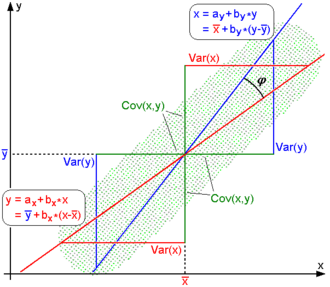
Regression lines for y = g _X (ten) [ruby-red] and x = g _Y (y) [blue]

For uncentered data, at that place is a relation between the correlation coefficient and the bending φ between the two regression lines, y = g _X (10) and x = m _Y (y), obtained by regressing y on x and x on y respectively. (Here, φ is measured counterclockwise within the first quadrant formed around the lines' intersection point if r > 0, or counterclockwise from the fourth to the 2nd quadrant if r < 0.) One tin show^[17] that if the standard deviations are equal, then r = sec φ − tan φ , where sec and tan are trigonometric functions.

For centered information (i.e., information which take been shifted past the sample means of their respective variables so every bit to have an average of cipher for each variable), the correlation coefficient can also be viewed as the cosine of the angle θ between the two observed vectors in Northward-dimensional space (for Northward observations of each variable)^[18]

Both the uncentered (non-Pearson-compliant) and centered correlation coefficients can be determined for a dataset. Equally an example, suppose 5 countries are plant to have gross national products of 1, 2, three, 5, and 8 billion dollars, respectively. Suppose these aforementioned five countries (in the aforementioned lodge) are found to take eleven%, 12%, thirteen%, 15%, and xviii% poverty. Then let x and y be ordered 5-element vectors containing the to a higher place data: 10 = (1, ii, iii, 5, 8) and y = (0.xi, 0.12, 0.thirteen, 0.15, 0.18).

By the usual process for finding the angle θ between two vectors (come across dot production), the uncentered correlation coefficient is:

${\displaystyle \cos \theta ={\frac {\mathbf {x} \cdot \mathbf {y} }{\left\|\mathbf {ten} \right\|\left\|\mathbf {y} \correct\|}}={\frac {2.93}{{\sqrt {103}}{\sqrt {0.0983}}}}=0.920814711.}$

This uncentered correlation coefficient is identical with the cosine similarity. Note that the above data were deliberately called to be perfectly correlated: y = 0.10 + 0.01 x . The Pearson correlation coefficient must therefore be exactly one. Centering the information (shifting x by ℰ(x) = 3.8 and y by ℰ(y) = 0.138) yields x = (−2.eight, −1.8, −0.8, 1.two, iv.2) and y = (−0.028, −0.018, −0.008, 0.012, 0.042), from which

${\displaystyle \cos \theta ={\frac {\mathbf {x} \cdot \mathbf {y} }{\left\|\mathbf {x} \right\|\left\|\mathbf {y} \right\|}}={\frac {0.308}{{\sqrt {30.8}}{\sqrt {0.00308}}}}=1=\rho _{xy},}$

as expected.

Estimation of the size of a correlation [edit]

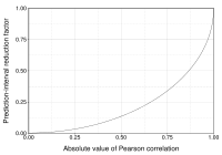
This figure gives a sense of how the usefulness of a Pearson correlation for predicting values varies with its magnitude. Given jointly normal X, Y with correlation ρ, ${\displaystyle ane-{\sqrt {1-\rho ^{2}}}}$ (plotted hither as a part of ρ) is the gene by which a given prediction interval for Y may be reduced given the corresponding value of Ten. For example, if ρ = 0.5, then the 95% prediction interval of Y|Ten volition exist about 13% smaller than the 95% prediction interval of Y.

Several authors have offered guidelines for the interpretation of a correlation coefficient.^{[xix] [twenty]} Nonetheless, all such criteria are in some ways capricious.^[20] The interpretation of a correlation coefficient depends on the context and purposes. A correlation of 0.8 may be very depression if one is verifying a physical law using high-quality instruments, but may be regarded as very high in the social sciences, where there may be a greater contribution from complicating factors.

Inference [edit]

Statistical inference based on Pearson's correlation coefficient oft focuses on one of the post-obit 2 aims:

• One aim is to test the cipher hypothesis that the true correlation coefficient ρ is equal to 0, based on the value of the sample correlation coefficient r.
• The other aim is to derive a confidence interval that, on repeated sampling, has a given probability of containing ρ.

Nosotros discuss methods of achieving 1 or both of these aims below.

Using a permutation test [edit]

Permutation tests provide a straight approach to performing hypothesis tests and constructing confidence intervals. A permutation test for Pearson's correlation coefficient involves the post-obit two steps:

1. Using the original paired data (x _i ,y _i ), randomly redefine the pairs to create a new data set (x _i ,y _i′ ), where the i′ are a permutation of the set {i,...,due north}. The permutation i′ is selected randomly, with equal probabilities placed on all due north! possible permutations. This is equivalent to cartoon the i′ randomly without replacement from the set {1, ..., n}. In bootstrapping, a closely related approach, the i and the i′ are equal and drawn with replacement from {1, ..., due north};
2. Construct a correlation coefficient r from the randomized data.

To perform the permutation test, echo steps (ane) and (two) a large number of times. The p-value for the permutation test is the proportion of the r values generated in step (2) that are larger than the Pearson correlation coefficient that was calculated from the original data. Here "larger" tin mean either that the value is larger in magnitude, or larger in signed value, depending on whether a two-sided or one-sided test is desired.

Using a bootstrap [edit]

The bootstrap can be used to construct confidence intervals for Pearson's correlation coefficient. In the "non-parametric" bootstrap, due north pairs (ten _i ,y _i ) are resampled "with replacement" from the observed set of due north pairs, and the correlation coefficient r is calculated based on the resampled data. This procedure is repeated a large number of times, and the empirical distribution of the resampled r values are used to approximate the sampling distribution of the statistic. A 95% confidence interval for ρ tin can be divers as the interval spanning from the 2.5th to the 97.5th percentile of the resampled r values.

Standard error [edit]

If ${\displaystyle 10}$ and ${\displaystyle y}$ are random variables, a standard error is associated to the correlation in the null case is:

${\displaystyle \sigma _{r}={\sqrt {\frac {1-r^{two}}{n-2}}}}$

where ${\displaystyle r}$ is the correlation (assumed r≈0) and ${\displaystyle n}$ the sample size.^{[21] [22]}

Testing using Student'due south t-distribution [edit]

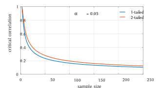
Disquisitional values of Pearson's correlation coefficient that must be exceeded to be considered significantly nonzero at the 0.05 level.

For pairs from an uncorrelated bivariate normal distribution, the sampling distribution of the studentized Pearson's correlation coefficient follows Student's t-distribution with degrees of liberty n − two. Specifically, if the underlying variables take a bivariate normal distribution, the variable

${\displaystyle t={\frac {r}{\sigma _{r}}}=r{\sqrt {\frac {n-two}{1-r^{ii}}}}}$

has a student's t-distribution in the nil instance (cypher correlation).^[23] This holds approximately in instance of non-normal observed values if sample sizes are big enough.^[24] For determining the critical values for r the inverse function is needed:

${\displaystyle r={\frac {t}{\sqrt {due north-2+t^{2}}}}.}$

Alternatively, large sample, asymptotic approaches can be used.

Some other early on paper^[25] provides graphs and tables for general values of ρ, for small sample sizes, and discusses computational approaches.

In the instance where the underlying variables are not normal, the sampling distribution of Pearson'due south correlation coefficient follows a Educatee's t-distribution, but the degrees of freedom are reduced.^[26]

Using the verbal distribution [edit]

For data that follow a bivariate normal distribution, the exact density role f(r) for the sample correlation coefficient r of a normal bivariate is^{[27] [28] [29]}

${\displaystyle f(r)={\frac {(n-ii)\,\mathrm {\Gamma } (n-1)(1-\rho ^{2})^{\frac {n-1}{two}}(one-r^{two})^{\frac {northward-iv}{2}}}{{\sqrt {2\pi }}\,\mathrm {\Gamma } (northward-{\tfrac {1}{two}})(1-\rho r)^{n-{\frac {iii}{2}}}}}{}_{ii}\mathrm {F} _{1}{\bigl (}{\tfrac {i}{two}},{\tfrac {i}{ii}};{\tfrac {one}{2}}(2n-one);{\tfrac {i}{2}}(\rho r+ane){\bigr )}}$

where ${\displaystyle \Gamma }$ is the gamma function and ${\displaystyle {}_{2}\mathrm {F} _{1}(a,b;c;z)}$ is the Gaussian hypergeometric role.

In the special instance when ${\displaystyle \rho =0}$ (naught population correlation), the exact density role f(r) can be written every bit:

${\displaystyle f(r)={\frac {\left(ane-r^{2}\right)^{\frac {northward-4}{two}}}{\mathrm {B} \left({\tfrac {i}{2}},{\tfrac {1}{2}}(due north-ii)\right)}},}$

where ${\displaystyle \mathrm {B} }$ is the beta function, which is one way of writing the density of a Student'south t-distribution, every bit higher up.

Using the verbal confidence distribution [edit]

Confidence intervals and tests can be calculated from a conviction distribution. An exact confidence density for ρ is^[30]

$${\displaystyle \pi (\rho |r)={\frac {\nu (\nu -ane)\Gamma (\nu -one)}{{\sqrt {2\pi }}\Gamma (\nu +{\frac {one}{2}})}}(1-r^{2})^{\frac {\nu -ane}{2}}\cdot (one-\rho ^{2})^{\frac {\nu -2}{2}}\cdot (one-r\rho )^{\frac {ane-2\nu }{ii}}F\left({\tfrac {3}{2}},-{\tfrac {1}{2}};\nu +{\tfrac {1}{2}};{\tfrac {i+r\rho }{2}}\right)}$$

where ${\displaystyle F}$ is the Gaussian hypergeometric function and ${\displaystyle \nu =n-1>ane}$ .

Using the Fisher transformation [edit]

In practice, confidence intervals and hypothesis tests relating to ρ are usually carried out using the Fisher transformation, ${\displaystyle F}$ :

${\displaystyle F(r)\equiv {\tfrac {i}{2}}\,\ln \left({\frac {1+r}{1-r}}\right)=\operatorname {artanh} (r)}$

F(r) approximately follows a normal distribution with

${\displaystyle {\text{mean}}=F(\rho )=\operatorname {artanh} (\rho )}$ and standard error ${\displaystyle ={\text{SE}}={\frac {1}{\sqrt {n-3}}},}$

where north is the sample size. The approximation mistake is everyman for a large sample size ${\displaystyle n}$ and small ${\displaystyle r}$ and ${\displaystyle \rho _{0}}$ and increases otherwise.

Using the approximation, a z-score is

${\displaystyle z={\frac {ten-{\text{mean}}}{\text{SE}}}=[F(r)-F(\rho _{0})]{\sqrt {n-3}}}$

under the naught hypothesis that ${\displaystyle \rho =\rho _{0}}$ , given the assumption that the sample pairs are independent and identically distributed and follow a bivariate normal distribution. Thus an approximate p-value can be obtained from a normal probability tabular array. For case, if z = two.2 is observed and a two-sided p-value is desired to test the goose egg hypothesis that ${\displaystyle \rho =0}$ , the p-value is 2 Φ(−two.2) = 0.028, where Φ is the standard normal cumulative distribution role.

To obtain a confidence interval for ρ, we first compute a confidence interval for F( ${\displaystyle \rho }$ ):

${\displaystyle 100(1-\alpha )\%{\text{CI}}:\operatorname {artanh} (\rho )\in [\operatorname {artanh} (r)\pm z_{\alpha /two}{\text{SE}}]}$

The inverse Fisher transformation brings the interval back to the correlation scale.

${\displaystyle 100(1-\blastoff )\%{\text{CI}}:\rho \in [\tanh(\operatorname {artanh} (r)-z_{\blastoff /2}{\text{SE}}),\tanh(\operatorname {artanh} (r)+z_{\alpha /2}{\text{SE}})]}$

For instance, suppose we find r = 0.3 with a sample size of n=50, and we wish to obtain a 95% confidence interval for ρ. The transformed value is arctanh(r) = 0.30952, and so the conviction interval on the transformed scale is 0.30952 ± one.96/√47 , or (0.023624, 0.595415). Converting dorsum to the correlation scale yields (0.024, 0.534).

In least squares regression assay [edit]

The square of the sample correlation coefficient is typically denoted r ² and is a special case of the coefficient of determination. In this case, it estimates the fraction of the variance in Y that is explained by X in a unproblematic linear regression. And then if we have the observed dataset ${\displaystyle Y_{i},\dots ,Y_{north}}$ and the fitted dataset ${\displaystyle {\chapeau {Y}}_{1},\dots ,{\hat {Y}}_{n}}$ then every bit a starting indicate the total variation in the Y _i around their boilerplate value tin can be decomposed as follows

${\displaystyle \sum _{i}(Y_{i}-{\bar {Y}})^{2}=\sum _{i}(Y_{i}-{\hat {Y}}_{i})^{2}+\sum _{i}({\lid {Y}}_{i}-{\bar {Y}})^{2},}$

where the ${\displaystyle {\hat {Y}}_{i}}$ are the fitted values from the regression analysis. This tin can be rearranged to give

${\displaystyle 1={\frac {\sum _{i}(Y_{i}-{\chapeau {Y}}_{i})^{2}}{\sum _{i}(Y_{i}-{\bar {Y}})^{two}}}+{\frac {\sum _{i}({\hat {Y}}_{i}-{\bar {Y}})^{2}}{\sum _{i}(Y_{i}-{\bar {Y}})^{2}}}.}$

The ii summands to a higher place are the fraction of variance in Y that is explained by X (right) and that is unexplained by X (left).

Next, we apply a property of least square regression models, that the sample covariance between ${\displaystyle {\hat {Y}}_{i}}$ and ${\displaystyle Y_{i}-{\hat {Y}}_{i}}$ is null. Thus, the sample correlation coefficient between the observed and fitted response values in the regression tin can be written (calculation is under expectation, assumes Gaussian statistics)

${\displaystyle {\begin{aligned}r(Y,{\hat {Y}})&={\frac {\sum _{i}(Y_{i}-{\bar {Y}})({\lid {Y}}_{i}-{\bar {Y}})}{\sqrt {\sum _{i}(Y_{i}-{\bar {Y}})^{2}\cdot \sum _{i}({\hat {Y}}_{i}-{\bar {Y}})^{2}}}}\\[6pt]&={\frac {\sum _{i}(Y_{i}-{\hat {Y}}_{i}+{\hat {Y}}_{i}-{\bar {Y}})({\lid {Y}}_{i}-{\bar {Y}})}{\sqrt {\sum _{i}(Y_{i}-{\bar {Y}})^{2}\cdot \sum _{i}({\hat {Y}}_{i}-{\bar {Y}})^{two}}}}\\[6pt]&={\frac {\sum _{i}[(Y_{i}-{\lid {Y}}_{i})({\lid {Y}}_{i}-{\bar {Y}})+({\hat {Y}}_{i}-{\bar {Y}})^{2}]}{\sqrt {\sum _{i}(Y_{i}-{\bar {Y}})^{2}\cdot \sum _{i}({\hat {Y}}_{i}-{\bar {Y}})^{2}}}}\\[6pt]&={\frac {\sum _{i}({\hat {Y}}_{i}-{\bar {Y}})^{2}}{\sqrt {\sum _{i}(Y_{i}-{\bar {Y}})^{2}\cdot \sum _{i}({\hat {Y}}_{i}-{\bar {Y}})^{ii}}}}\\[6pt]&={\sqrt {\frac {\sum _{i}({\hat {Y}}_{i}-{\bar {Y}})^{2}}{\sum _{i}(Y_{i}-{\bar {Y}})^{2}}}}.\finish{aligned}}}$

Thus

${\displaystyle r(Y,{\lid {Y}})^{2}={\frac {\sum _{i}({\lid {Y}}_{i}-{\bar {Y}})^{2}}{\sum _{i}(Y_{i}-{\bar {Y}})^{2}}}}$

where ${\displaystyle r(Y,{\hat {Y}})^{2}}$ is the proportion of variance in Y explained by a linear office of 10.

In the derivation in a higher place, the fact that

${\displaystyle \sum _{i}(Y_{i}-{\lid {Y}}_{i})({\lid {Y}}_{i}-{\bar {Y}})=0}$

can be proved past noticing that the fractional derivatives of the rest sum of squares (RSS) over β ₀ and β _i are equal to 0 in the least squares model, where

${\displaystyle {\text{RSS}}=\sum _{i}(Y_{i}-{\hat {Y}}_{i})^{2}}$ .

In the finish, the equation can be written as:

${\displaystyle r(Y,{\hat {Y}})^{2}={\frac {{\text{SS}}_{\text{reg}}}{{\text{SS}}_{\text{tot}}}}}$

where

The symbol ${\displaystyle {\text{SS}}_{\text{reg}}}$ is chosen the regression sum of squares, also called the explained sum of squares, and ${\displaystyle {\text{SS}}_{\text{tot}}}$ is the total sum of squares (proportional to the variance of the data).

Sensitivity to the data distribution [edit]

Beingness [edit]

The population Pearson correlation coefficient is defined in terms of moments, and therefore exists for whatsoever bivariate probability distribution for which the population covariance is defined and the marginal population variances are defined and are not-nil. Some probability distributions, such equally the Cauchy distribution, have undefined variance and hence ρ is not defined if 10 or Y follows such a distribution. In some practical applications, such as those involving data suspected to follow a heavy-tailed distribution, this is an important consideration. However, the being of the correlation coefficient is commonly not a business; for example, if the range of the distribution is bounded, ρ is always divers.

Sample size [edit]

• If the sample size is moderate or large and the population is normal, and then, in the case of the bivariate normal distribution, the sample correlation coefficient is the maximum likelihood estimate of the population correlation coefficient, and is asymptotically unbiased and efficient, which roughly means that it is impossible to construct a more accurate estimate than the sample correlation coefficient.
• If the sample size is big and the population is not normal, then the sample correlation coefficient remains approximately unbiased, only may not be efficient.
• If the sample size is large, and then the sample correlation coefficient is a consequent estimator of the population correlation coefficient as long equally the sample means, variances, and covariance are consistent (which is guaranteed when the law of large numbers can be applied).
• If the sample size is pocket-sized, and so the sample correlation coefficient r is not an unbiased estimate of ρ.^[10] The adjusted correlation coefficient must be used instead: see elsewhere in this commodity for the definition.
• Correlations tin can be dissimilar for imbalanced dichotomous data when there is variance error in sample.^[31]

Robustness [edit]

Like many commonly used statistics, the sample statistic r is not robust,^[32] so its value can exist misleading if outliers are present.^{[33] [34]} Specifically, the PMCC is neither distributionally robust,^{[ commendation needed ]} nor outlier resistant^[32] (run across Robust statistics § Definition). Inspection of the scatterplot between X and Y volition typically reveal a situation where lack of robustness might be an upshot, and in such cases it may exist advisable to apply a robust measure of association. Note however that while most robust estimators of association measure out statistical dependence in some style, they are more often than not not interpretable on the same scale as the Pearson correlation coefficient.

Statistical inference for Pearson'south correlation coefficient is sensitive to the data distribution. Exact tests, and asymptotic tests based on the Fisher transformation can exist applied if the data are approximately usually distributed, simply may be misleading otherwise. In some situations, the bootstrap can exist practical to construct conviction intervals, and permutation tests can be applied to carry out hypothesis tests. These non-parametric approaches may give more meaningful results in some situations where bivariate normality does not hold. Withal the standard versions of these approaches rely on exchangeability of the information, significant that there is no ordering or grouping of the information pairs being analyzed that might affect the behavior of the correlation judge.

A stratified assay is one way to either adapt a lack of bivariate normality, or to isolate the correlation resulting from one cistron while controlling for another. If W represents cluster membership or some other factor that information technology is desirable to command, nosotros tin stratify the data based on the value of Westward, then summate a correlation coefficient inside each stratum. The stratum-level estimates tin then exist combined to gauge the overall correlation while controlling for West.^[35]

Variants [edit]

Variations of the correlation coefficient tin be calculated for dissimilar purposes. Here are some examples.

Adapted correlation coefficient [edit]

The sample correlation coefficient r is not an unbiased gauge of ρ. For data that follows a bivariate normal distribution, the expectation Due east[r] for the sample correlation coefficient r of a normal bivariate is^[36]

${\displaystyle \operatorname {\mathbb {E} } \left[r\correct]=\rho -{\frac {\rho \left(1-\rho ^{two}\correct)}{2n}}+\cdots ,\quad }$ therefore r is a biased estimator of ${\displaystyle \rho .}$

The unique minimum variance unbiased estimator r _adj is given by^[37]

${\displaystyle r_{\text{adj}}=r\,\mathbf {_{2}F_{one}} \left({\frac {1}{2}},{\frac {1}{2}};{\frac {northward-1}{2}};1-r^{2}\right),}$

(1)

where:

An approximately unbiased reckoner r _adj can exist obtained^{[ citation needed ]} by truncating E[r] and solving this truncated equation:

${\displaystyle r=\operatorname {\mathbb {Eastward} } [r]\approx r_{\text{adj}}-{\frac {r_{\text{adj}}(i-r_{\text{adj}}^{2})}{2n}}.}$

(ii)

An guess solution^{[ citation needed ]} to equation (2) is:

${\displaystyle r_{\text{adj}}\approx r\left[1+{\frac {ane-r^{two}}{2n}}\right],}$

(iii)

where in (3):

• ${\displaystyle r,n}$ are defined as above,
• r _adj is a suboptimal estimator,^{[ citation needed ] [ clarification needed ]}
• r _adj can too exist obtained past maximizing log(f(r)),
• r _adj has minimum variance for large values of due north,
• r _adj has a bias of guild 1⁄(n − one) .

Another proposed^[x] adjusted correlation coefficient is:^{[ citation needed ]}

${\displaystyle r_{\text{adj}}={\sqrt {one-{\frac {(one-r^{2})(n-ane)}{(north-ii)}}}}.}$

Notation that r _adj ≈ r for large values ofn.

Weighted correlation coefficient [edit]

Suppose observations to be correlated take differing degrees of importance that can be expressed with a weight vector w. To calculate the correlation between vectors 10 and y with the weight vector west (all of lengthdue north),^{[38] [39]}

• Weighted hateful:

  $${\displaystyle \operatorname {k} (x;westward)={\frac {\sum _{i}w_{i}x_{i}}{\sum _{i}w_{i}}}.}$$

  

• Weighted covariance

  $${\displaystyle \operatorname {cov} (x,y;w)={\frac {\sum _{i}w_{i}\cdot (x_{i}-\operatorname {g} (x;due west))(y_{i}-\operatorname {m} (y;w))}{\sum _{i}w_{i}}}.}$$

  

• Weighted correlation

  $${\displaystyle \operatorname {corr} (ten,y;west)={\frac {\operatorname {cov} (10,y;w)}{\sqrt {\operatorname {cov} (x,x;w)\operatorname {cov} (y,y;w)}}}.}$$

  

Cogitating correlation coefficient [edit]

The cogitating correlation is a variant of Pearson'south correlation in which the information are not centered around their hateful values.^{[ citation needed ]} The population reflective correlation is

${\displaystyle \operatorname {corr} _{r}(X,Y)={\frac {\operatorname {\mathbb {E} } [\,X\,Y\,]}{\sqrt {\operatorname {\mathbb {Due east} } [\,10^{2}\,]\cdot \operatorname {\mathbb {E} } [\,Y^{2}\,]}}}.}$

The reflective correlation is symmetric, only information technology is not invariant nether translation:

${\displaystyle \operatorname {corr} _{r}(10,Y)=\operatorname {corr} _{r}(Y,X)=\operatorname {corr} _{r}(10,bY)\neq \operatorname {corr} _{r}(X,a+by),\quad a\neq 0,b>0.}$

The sample cogitating correlation is equivalent to cosine similarity:

${\displaystyle rr_{xy}={\frac {\sum x_{i}y_{i}}{\sqrt {(\sum x_{i}^{2})(\sum y_{i}^{2})}}}.}$

The weighted version of the sample reflective correlation is

${\displaystyle rr_{xy,w}={\frac {\sum w_{i}x_{i}y_{i}}{\sqrt {(\sum w_{i}x_{i}^{two})(\sum w_{i}y_{i}^{2})}}}.}$

Scaled correlation coefficient [edit]

Scaled correlation is a variant of Pearson'due south correlation in which the range of the data is restricted intentionally and in a controlled manner to reveal correlations betwixt fast components in time series.^[40] Scaled correlation is defined as boilerplate correlation across curt segments of data.

Let ${\displaystyle K}$ be the number of segments that tin can fit into the total length of the signal ${\displaystyle T}$ for a given scale ${\displaystyle s}$ :

${\displaystyle 1000=\operatorname {round} \left({\frac {T}{southward}}\right).}$

The scaled correlation across the unabridged signals ${\displaystyle {\bar {r}}_{s}}$ is and so computed every bit

${\displaystyle {\bar {r}}_{s}={\frac {one}{Chiliad}}\sum \limits _{k=1}^{K}r_{chiliad},}$

where ${\displaystyle r_{k}}$ is Pearson'south coefficient of correlation for segment ${\displaystyle k}$ .

By choosing the parameter ${\displaystyle s}$ , the range of values is reduced and the correlations on long time scale are filtered out, simply the correlations on short time scales being revealed. Thus, the contributions of slow components are removed and those of fast components are retained.

Pearson's altitude [edit]

A distance metric for ii variables X and Y known every bit Pearson's altitude tin be defined from their correlation coefficient as^[41]

${\displaystyle d_{X,Y}=1-\rho _{10,Y}.}$

Considering that the Pearson correlation coefficient falls between [−one, +1], the Pearson distance lies in [0, 2]. The Pearson distance has been used in cluster assay and data detection for communications and storage with unknown gain and beginning.^[42]

The Pearson "altitude" defined this manner assigns distance greater than 1 to negative correlations. In reality, both strong positive correlation and negative correlations are meaningful, and so intendance must be taken when Pearson "altitude" is used for nearest neighbor algorithm as such algorithm will just include neighbors with positive correlation and exclude neighbors with negative correlation. Alternatively, an accented valued distance: ${\displaystyle d_{X,Y}=i-|\rho _{X,Y}|}$ can exist applied, which will have both positive and negative correlations into consideration. The data on positive and negative association can be extracted separately, later.

Circular correlation coefficient [edit]

For variables X = {x _ane,...,x _n } and Y = {y ₁,...,y _n } that are defined on the unit circle [0, 2π), information technology is possible to define a circular analog of Pearson's coefficient.^[43] This is done by transforming information points in 10 and Y with a sine function such that the correlation coefficient is given every bit:

${\displaystyle r_{\text{round}}={\frac {\sum _{i=one}^{due north}\sin(x_{i}-{\bar {ten}})\sin(y_{i}-{\bar {y}})}{{\sqrt {\sum _{i=1}^{north}\sin(x_{i}-{\bar {x}})^{2}}}{\sqrt {\sum _{i=1}^{n}\sin(y_{i}-{\bar {y}})^{ii}}}}}}$

where ${\displaystyle {\bar {x}}}$ and ${\displaystyle {\bar {y}}}$ are the circular means of X andY. This measure out can exist useful in fields like meteorology where the angular direction of data is important.

Partial correlation [edit]

If a population or data-prepare is characterized past more than 2 variables, a partial correlation coefficient measures the forcefulness of dependence betwixt a pair of variables that is not accounted for by the mode in which they both alter in response to variations in a selected subset of the other variables.

Decorrelation of northward random variables [edit]

It is always possible to remove the correlations between all pairs of an arbitrary number of random variables by using a data transformation, even if the relationship betwixt the variables is nonlinear. A presentation of this result for population distributions is given by Cox & Hinkley.^[44]

A corresponding result exists for reducing the sample correlations to zero. Suppose a vector of n random variables is observed m times. Permit X exist a matrix where ${\displaystyle X_{i,j}}$ is the jth variable of ascertainment i. Permit ${\displaystyle Z_{yard,m}}$ be an thou by m square matrix with every chemical element one. So D is the information transformed then every random variable has goose egg mean, and T is the data transformed so all variables have null mean and zero correlation with all other variables – the sample correlation matrix of T will be the identity matrix. This has to exist farther divided by the standard deviation to get unit variance. The transformed variables volition be uncorrelated, even though they may non exist independent.

${\displaystyle D=X-{\frac {1}{m}}Z_{g,1000}Ten}$

${\displaystyle T=D(D^{\mathsf {T}}D)^{-{\frac {1}{2}}},}$

where an exponent of −+ i⁄2 represents the matrix square root of the inverse of a matrix. The correlation matrix of T will be the identity matrix. If a new data ascertainment ten is a row vector of due north elements, then the same transform tin be applied to ten to get the transformed vectors d and t:

${\displaystyle d=x-{\frac {i}{m}}Z_{i,m}X,}$

${\displaystyle t=d(D^{\mathsf {T}}D)^{-{\frac {1}{two}}}.}$

This decorrelation is related to principal components analysis for multivariate information.

Software implementations [edit]

• R's statistics base of operations-package implements the correlation coefficient with cor(x, y), or (with the P value also) with cor.exam(x, y).
• The SciPy Python library via pearsonr(10, y).
• The Pandas Python library implements Pearson correlation coefficient calculation as the default option for the method pandas.DataFrame.corr
• Wolfram Mathematica via the Correlation function, or (with the P value) with CorrelationTest.
• The Heave C++ library via the correlation_coefficient function.

See also [edit]

• Anscombe'due south quartet
• Association (statistics)
• Coefficient of colligation
  • Yule'southward Q
  • Yule's Y
• Concordance correlation coefficient
• Correlation and dependence
• Correlation ratio
• Disattenuation
• Distance correlation
• Maximal information coefficient
• Multiple correlation
• Ordinarily distributed and uncorrelated does non imply independent
• Odds ratio
• Partial correlation
• Polychoric correlation
• Quadrant count ratio
• RV coefficient
• Spearman's rank correlation coefficient

Footnotes [edit]

1. ^ As early as 1877, Galton was using the term "reversion" and the symbol "r" for what would become "regression".^{[3] [4] [5]}

References [edit]

1. ^ "SPSS Tutorials: Pearson Correlation".
2. ^ "Correlation Coefficient: Uncomplicated Definition, Formula, Piece of cake Steps". Statistics How To.
3. ^ Galton, F. (v–nineteen April 1877). "Typical laws of heredity". Nature. xv (388, 389, 390): 492–495, 512–514, 532–533. Bibcode:1877Natur..fifteen..492.. doi:10.1038/015492a0. S2CID 4136393. In the "Appendix" on page 532, Galton uses the term "reversion" and the symbol r.
4. ^ Galton, F. (24 September 1885). "The British Association: Section II, Anthropology: Opening address by Francis Galton, F.R.South., etc., President of the Anthropological Plant, President of the Department". Nature. 32 (830): 507–510.
5. ^ Galton, F. (1886). "Regression towards mediocrity in hereditary stature". Journal of the Anthropological Found of Cracking Britain and Ireland. 15: 246–263. doi:10.2307/2841583. JSTOR 2841583.
6. ^ Pearson, Karl (20 June 1895). "Notes on regression and inheritance in the example of 2 parents". Proceedings of the Regal Society of London. 58: 240–242. Bibcode:1895RSPS...58..240P.
7. ^ Stigler, Stephen M. (1989). "Francis Galton'southward account of the invention of correlation". Statistical Scientific discipline. 4 (2): 73–79. doi:10.1214/ss/1177012580. JSTOR 2245329.
8. ^ "Analyse mathematique sur les probabilités des erreurs de situation d'un betoken". Mem. Acad. Roy. Sci. Inst. French republic. Sci. Math, et Phys. (in French). ix: 255–332. 1844 – via Google Books.
9. ^ Wright, S. (1921). "Correlation and causation". Journal of Agricultural Research. 20 (7): 557–585.
10. ^ ^{a b c d east} Real Statistics Using Excel: Correlation: Basic Concepts, retrieved 22 February 2015
11. ^ Weisstein, Eric W. "Statistical Correlation". mathworld.wolfram.com . Retrieved 22 August 2020.
12. ^ Moriya, N. (2008). "Noise-related multivariate optimal articulation-analysis in longitudinal stochastic processes". In Yang, Fengshan (ed.). Progress in Practical Mathematical Modeling. Nova Scientific discipline Publishers, Inc. pp. 223–260. ISBN978-1-60021-976-4.
13. ^ Garren, Steven T. (15 June 1998). "Maximum likelihood estimation of the correlation coefficient in a bivariate normal model, with missing information". Statistics & Probability Letters. 38 (3): 281–288. doi:10.1016/S0167-7152(98)00035-2.
14. ^ "2.6 - (Pearson) Correlation Coefficient r". STAT 462 . Retrieved 10 July 2021.
15. ^ "Introductory Business organisation Statistics: The Correlation Coefficient r". opentextbc.ca . Retrieved 21 August 2020.
16. ^ Rodgers; Nicewander (1988). "Thirteen ways to look at the correlation coefficient" (PDF). The American Statistician. 42 (i): 59–66. doi:10.2307/2685263. JSTOR 2685263.
17. ^ Schmid, John Jr. (December 1947). "The relationship between the coefficient of correlation and the angle included between regression lines". The Journal of Educational Research. 41 (4): 311–313. doi:ten.1080/00220671.1947.10881608. JSTOR 27528906.
18. ^ Rummel, R.J. (1976). "Understanding Correlation". ch. 5 (as illustrated for a special case in the adjacent paragraph).
19. ^ Buda, Andrzej; Jarynowski, Andrzej (December 2010). Life Time of Correlations and its Applications. Wydawnictwo Niezależne. pp. five–21. ISBN9788391527290.
20. ^ ^{a b} Cohen, J. (1988). Statistical Ability Assay for the Behavioral Sciences (2nd ed.).
21. ^ Bowley, A. 50. (1928). "The Standard Deviation of the Correlation Coefficient". Journal of the American Statistical Clan. 23 (161): 31–34. doi:10.2307/2277400. ISSN 0162-1459. JSTOR 2277400.
22. ^ "Derivation of the standard mistake for Pearson's correlation coefficient". Cross Validated . Retrieved thirty July 2021.
23. ^ Rahman, N. A. (1968) A Form in Theoretical Statistics, Charles Griffin and Company, 1968
24. ^ Kendall, G. Thousand., Stuart, A. (1973) The Advanced Theory of Statistics, Volume 2: Inference and Relationship, Griffin. ISBN 0-85264-215-half dozen (Section 31.19)
25. ^ Soper, H.E.; Young, A.W.; Cavern, B.M.; Lee, A.; Pearson, Thou. (1917). "On the distribution of the correlation coefficient in minor samples. Appendix Two to the papers of "Educatee" and R.A. Fisher. A co-operative study". Biometrika. eleven (iv): 328–413. doi:ten.1093/biomet/11.iv.328.
26. ^ Davey, Catherine E.; Grayden, David B.; Egan, Gary F.; Johnston, Leigh A. (January 2013). "Filtering induces correlation in fMRI resting state data". NeuroImage. 64: 728–740. doi:10.1016/j.neuroimage.2012.08.022. hdl:11343/44035. PMID 22939874. S2CID 207184701.
27. ^ Hotelling, Harold (1953). "New Light on the Correlation Coefficient and its Transforms". Periodical of the Royal Statistical Society. Serial B (Methodological). 15 (2): 193–232. doi:10.1111/j.2517-6161.1953.tb00135.x. JSTOR 2983768.
28. ^ Kenney, J.F.; Keeping, Due east.S. (1951). Mathematics of Statistics. Vol. Function 2 (second ed.). Princeton, NJ: Van Nostrand.
29. ^ Weisstein, Eric W. "Correlation Coefficient—Bivariate Normal Distribution". mathworld.wolfram.com.
30. ^ Taraldsen, Gunnar (2020). "Confidence in Correlation". doi:10.13140/RG.two.2.23673.49769.
31. ^ Lai, Chun Sing; Tao, Yingshan; Xu, Fangyuan; Ng, Wing Due west.Y.; Jia, Youwei; Yuan, Haoliang; Huang, Chao; Lai, Loi Lei; Xu, Zhao; Locatelli, Giorgio (January 2019). "A robust correlation analysis framework for imbalanced and dichotomous data with uncertainty" (PDF). Information Sciences. 470: 58–77. doi:ten.1016/j.ins.2018.08.017. S2CID 52878443.
32. ^ ^{a b} Wilcox, Rand R. (2005). Introduction to robust estimation and hypothesis testing. Academic Press.
33. ^ Devlin, Susan J.; Gnanadesikan, R.; Kettenring J.R. (1975). "Robust estimation and outlier detection with correlation coefficients". Biometrika. 62 (3): 531–545. doi:10.1093/biomet/62.three.531. JSTOR 2335508.
34. ^ Huber, Peter. J. (2004). Robust Statistics. Wiley. ^{[ page needed ]}
35. ^ Katz., Mitchell H. (2006) Multivariable Analysis – A Applied Guide for Clinicians. 2d Edition. Cambridge University Printing. ISBN 978-0-521-54985-1. ISBN 0-521-54985-X
36. ^ Hotelling, H. (1953). "New Light on the Correlation Coefficient and its Transforms". Periodical of the Royal Statistical Society. Series B (Methodological). fifteen (2): 193–232. doi:10.1111/j.2517-6161.1953.tb00135.x. JSTOR 2983768.
37. ^ Olkin, Ingram; Pratt,John W. (March 1958). "Unbiased Estimation of Certain Correlation Coefficients". The Register of Mathematical Statistics. 29 (1): 201–211. doi:10.1214/aoms/1177706717. JSTOR 2237306. .
38. ^ "Re: Compute a weighted correlation". sci.tech-annal.net.
39. ^ "Weighted Correlation Matrix – File Substitution – MATLAB Primal".
40. ^ Nikolić, D; Muresan, RC; Feng, Due west; Singer, Westward (2012). "Scaled correlation analysis: a better way to compute a cantankerous-correlogram" (PDF). European Journal of Neuroscience. 35 (5): i–21. doi:10.1111/j.1460-9568.2011.07987.ten. PMID 22324876. S2CID 4694570.
41. ^ Fulekar (Ed.), M.H. (2009) Bioinformatics: Applications in Life and Environmental Sciences, Springer (pp. 110) ISBN 1-4020-8879-five
42. ^ Immink, K. Schouhamer; Weber, J. (October 2010). "Minimum Pearson distance detection for multilevel channels with gain and / or offset mismatch". IEEE Transactions on Data Theory. 60 (10): 5966–5974. CiteSeerX10.1.one.642.9971. doi:x.1109/tit.2014.2342744. S2CID 1027502. Retrieved 11 February 2018.
43. ^ Jammalamadaka, S. Rao; SenGupta, A. (2001). Topics in round statistics. New Bailiwick of jersey: Globe Scientific. p. 176. ISBN978-981-02-3778-3 . Retrieved 21 September 2016.
44. ^ Cox, D.R.; Hinkley, D.V. (1974). Theoretical Statistics. Chapman & Hall. Appendix 3. ISBN0-412-12420-3.

External links [edit]

• "cocor". comparingcorrelations.org. – A free spider web interface and R package for the statistical comparing of two dependent or independent correlations with overlapping or non-overlapping variables.
• "Correlation". nagysandor.eu. – an interactive Flash simulation on the correlation of ii normally distributed variables.
• "Correlation coefficient calculator". hackmath.net. Linear regression. –
• "Critical values for Pearson's correlation coefficient" (PDF). frank.mtsu.edu/~dkfuller. – big tabular array.
• "Judge the Correlation". – A game where players guess how correlated two variables in a besprinkle plot are, in order to proceeds a better understanding of the concept of correlation.

Non Linear Relationship Scatter Plot,

Source: https://en.wikipedia.org/wiki/Pearson_correlation_coefficient

Posted by: wrightsagessay.blogspot.com

Share this post